1.  Introduction

Drivers on congested roads require information to allow them to make decisions as to whether to continue their journey, take a diversion, take a break or turn back. The Highways Agency has installed a system of variable message sites (VMS) along the motorway and trunk road network to provide information for drivers. In order to give information about delays and expected travel times it is necessary to make a reasonably accurate assessment of delay time. There are two ways of doing this:

1. Use the current and historic journey times;
2. Estimate the delay from the demand (number of vehicles wanting to use a stretch of road in a given time) and capacity (the number of vehicles able to traverse the stretch of road in a given time).

Journey times are derived from automatic number plate recognition (ANPR) cameras and are generally very accurate, but unfortunately they can only be applied retrospectively (i.e. they give accurate information about what has already happened). This is useful in a situation where the traffic flow and road capacity are reasonably stable. However, in a situation where the capacity is suddenly restricted so that it is less than the demand, the journey time method is of little use because vehicles joining a queue will, in general, experience a different delay to that experienced by the vehicles emerging from the queue (whose journey times are known). The method developed here uses the demand and capacity under dynamic conditions to inform drivers of vehicles joining the queue what delay they should expect.

2.  Background

The National Traffic Control Centre (NTCC) is run by Serco on behalf of the Highways Agency (HA). It collects traffic data that could be used for calculating delays in two principal ways.

1. Journey times are calculated from ANPR camera data. An upstream camera recognises a number plate and converts it to a coded form. If a downstream camera detects the same number plate, it will generate the same code, which is known as a match. There are some erroneous matches because the code is not unique, but in practice this causes few problems. Once a match is established the computer systems calculate the journey time and use this to produce an average journey time between two points on the road network.
2. Traffic flows are calculated from induction loop data. The induction loops are buried in the road and count the vehicles that pass over them. In addition they can detect vehicle speed, length and carriageway occupancy (the percentage of the road covered by vehicles). The NTCC system calculates flows as vehicles per hour (vph) every five minutes. It does this by counting the vehicles that passed over a loop site in the previous ten minutes and multiplying the total by 6. The induction loops are known as monitoring sites.

The VEDENS[1] traffic flow simulation has been used extensively by NTCC to establish the requirements to produce accurate traffic flow data and to assess the way in which density waves propagate along a carriageway. It has also been used to assess the capacity of various road geometries. The code simulates the collection of traffic date via induction loops and ANPR cameras.

3.  Outline of the Model

Consider a stretch of road where the upstream monitored flow is U and the downstream monitored flow is D. Assume the simple case that all the traffic passing the upstream monitor also passes the downstream monitor (i.e. no vehicles join or leave the carriageway). As long as there is no restriction in capacity, U and D can vary and there will be no congestion. However, if there is a capacity restriction C, caused either by the road geometry or an event, such as an accident, then D will be limited to C. The result is that there will be congestion, which we may regard as a nascent queue. There will be a net accumulation of vehicles within the stretch of road. The net accumulation of vehicles, Q(n), in n equal time intervals of δt, is given by:

Clearly Q will increase in cases where U_i > D_i , whereas when D_i > U_i , Q will decrease. Q is actually equal to the number of vehicles on the stretch of road between the upstream and downstream monitoring sites. At time n, the rate of flow out of the stretch of road is D_n, so if U_i and D_i are expressed in vehicles per hour (vph) the time T(n) for each vehicle to traverse the stretch of road is Q/D_n. At NTCC, the traffic flow data are reported every 5 minutes, so equating t to 5 minutes we can derive T(n) (expressed in minutes)

It should be noted that there is no reference to either speed or distance in Equation 2. In effect it is a queuing model, with the time taken for a vehicle at the start of the stretch of road (the back of the queue) to reach the end of the stretch of road (the front of the queue) equal to the number of vehicles in the queue divided by the downstream rate of flow (the rate at which the queue is emptied).

4.  Calculations

Equation 2 has been applie2 to calculations carried out using the VEDENS code[1]. The input data were configured so that flow data and journey times were collected every five minutes, to mimic the NTCC system. The journey time between two points was calculated by back fitting and matching the start time for the two points.

For this simple example, a constant demand flow of 3000 vph on one carriageway of a 2-lane dual carriageway was assumed. A typical mixture of vehicle types and driver characteristics was used. The simulation was allowed to equilibrate for 2 hours simulation time prior to starting the time-recording clock and then a further 2 hours was allowed to elapse in order to establish profile journey times. The scenario comprised 60 km of carriageway with a loop-based monitoring site every 5 km (6 km in the case of the final loop site). The first 5 km was to allow the traffic to assume a totally random configuration prior to the sections used for the calculations. The final 4 km was to ensure vehicles continued in a normal manner after the completing the sections used for the calculations.

There was an ANPR monitoring facility at each monitoring site and the delay information is that which could be delivered via a VMS located at each monitoring site. After the initial period during which the journey time profiles were established, Lane 2 was blocked as though by an accident or breakdown. The site of the blockage was 50 km downstream from the first monitoring site and 100 m of carriageway prior to the blockage site was assumed to be unusable (as though coned off). The final monitoring site and ANPR camera were 1 km downstream from the site of the blockage. The blockage was allowed to persist for 3 hours, after which time the road was clear and normal flow was allowed to resume. The simulation continued for a further 5 hours so that the traffic flow could return to its normal state.

5.  Results

The main results are shown in Figures 1 to 6. In each case the blue bar represents the additional delay yet to be experienced by a driver at the given point on the road. The green bar represents the delay prediction that could be given to drivers, based on Equation 2. The red bar represents the delay prediction based on the latest journey time information available at the time a driver passed a monitoring site. In each case the delay is the additional time taken to reach the final monitoring section compared with the profile (ideal) time calculated during the first two hours.

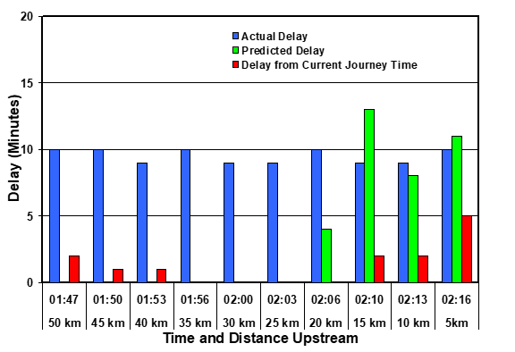
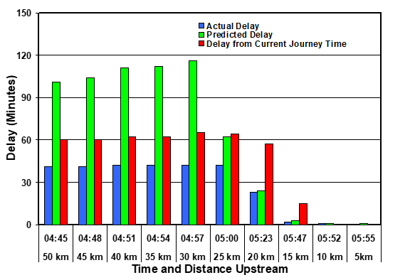
Figure 1 shows the situation for drivers who reached the final monitoring site at 02:30 (00:00 represents the starting of the time-recording clock). The blue bars indicate the delay that was actually experienced between the upstream monitoring site and the final monitoring site. These were, of course entirely unpredictable prior to 02:00, the time at which the blockage occurred. However, by 02:05, while the drivers were still more than 20km upstream, a delay would have been generated by the methodology of Equation 2 indicating a delay 20km away. By 02:10, when the drivers were 15 km upstream, the delay would have been fully predicted (actually somewhat over-predicted). Thereafter the predictions would have been very accurate. If, instead of using Equation 2, the latest journey time information had been used to predict the delay, it would have been triggered late and would have seriously under-estimated the delay.

Figure 2 illustrates the situation for drivers reaching the final monitoring site at 03:30. In this case the blockage occurred while drivers were more than 50 km upstream and so there would have been adequate warning of the delay, even at this distance. The delay was initially somewhat under-estimated by Equation 2, but the prediction would have been sufficiently accurate for drivers to make an informed decision. On the other hand, a delay prediction based on the latest available journey time information would have seriously under-estimated the delay until drivers were well into the queue.

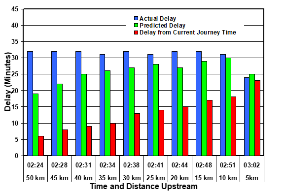
Figure 3 illustrates the situation for drivers reaching the final monitoring site at 04:30, half an hour before the blockage was cleared. In this case, there was a very good correspondence between the predictions of Equation 2 and the actual delay. On the other hand, the delay that would have been predicted by the latest available journey time would be extremely poor until the driver were at least half way through the queue.

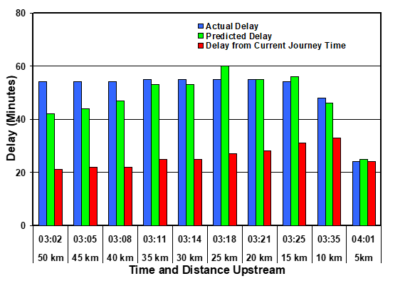
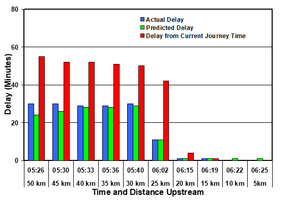
Figure 4 illustrates the situation for drivers reaching the final monitoring site at 05:30 (i.e. 30 minutes after the blockage was cleared).

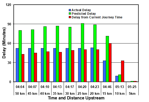
In this case the delay was over-predicted by Equation 2 up to the time that the blockage was removed. This is because there is no mechanism for detecting the clearance of the blockage prior to its actual clearance (i.e. there is no way to foretell the future). However, once the blockage was cleared the prediction of Equation 2 became very good. On the other hand, the prediction based on the latest available journey time was fortuitously good prior to the clearance of the blockage, but did not reflect the result of the clearance once it occurred.

Figure 5 illustrates the situation for drivers reaching the final monitoring site at 06:00. The situation depicted is similar to that of Figure 4 but, in this case, the blockage was cleared when the driver was 25 km upstream and thereafter the prediction of Equation 2 was very good.

Figures 1 to 5 clearly demonstrate that, when there is a discontinuity in the downstream flow, caused by an event such as the closing or opening of a lane, the application of Equation 2 will identify the change in delay as soon as the following 5-minute data is processed. On the other hand, the use of the latest journey time to make delay predictions cannot produce an accurate prediction until the flows have stabilised and returned to a steady state. In some circumstances this can take several hours.

Figure 6 illustrates the situation for drivers reaching the final monitoring site at 06:30. In this case the blockage was cleared while drivers were more than 50 km upstream and so there would have been adequate warning of the correct delay, even at this distance. The delay was predicted accurately by Equation 2 for the whole of the congested stretch of carriageway. On the other hand, a delay prediction based on the latest available journey time information would have seriously over-estimated the delay until drivers were past the congested stretch, in agreement with the above observations on Figures 1 to 5.

6.  Practical Requirements

The reported calculations were deliberately simplified to enable an evaluation of the basic methodology. However, for a practical system, three refinements need to be incorporated into the model:

1. The model needs to include an allowance for traffic joining or leaving the carriageway in such a way as to allow the net flow to change between monitoring sites;
2. The model needs to establish correct absolute values for the numbers of vehicles between each pair of monitoring sites;
3. The model needs to calculate the delay between each discrete pair of monitoring sites: the total delay would then be calculated as the aggregate of the delays between each two points on the route.

Net flow changes can be dealt with on the basis of mean flows. NTCC uses a methodology (known as LIP) that calculates the mean flows on each section of carriageway, based on 7 days of traffic data (2016 5-minute traffic flows). For two monitoring sites, we can regard the average flow at the upstream site as U and that at the downstream site as D. This means for every U vehicles passing the upstream monitoring point, D vehicles enter the "queue" to pass the downstream monitoring site. In this case the term "queue" simply means the number of vehicles that must pass the downstream monitoring point before a new vehicle passing the upstream monitoring point can reach the downstream monitoring site. So, when D_i vehicles pass the downstream monitoring point, (D/U).U_i vehicles will have entered the "queue". For Equation 2 to accurately predict the delay, based on the number of vehicles in the queue, it would then become

The correct absolute value for the number of vehicles between two monitoring sites was easily achieved in the simulation because at the start of the simulation there were no vehicles on the carriageway. The numbers remained correct because, in the simulation, the monitors were 100% efficient and recorded every vehicle with no false positives. However, in a practical loop-based system there will always be some over- and under-counting (although the loops are usually correct to within 1 or 2%).

There are two methods of establishing the correct absolute value for the number of vehicles between two monitoring sites in a practical situation. The simplest method is to reset the number to a pre-determined value at (say) 03:00 GMT every morning. At this time the number would be known to be low and could be calculated from the flow, average speed and distance between the monitoring sites. A slightly more sophisticated method would be to include reality checks by disallowing negative values and limiting the total number to equal about 100 vehicles per kilometre per lane.

The above refinements can be used to check the model against historical data for known blockage events.

7.  Conclusions

Equation 2 has been shown to produce the good predictions of downstream delay, based on known facts (i.e. it cannot take account of unplanned events that have not yet happened). There is a need to refine the model and check the validity of Equation 3 before it can be applied practically. The predictions for the effects of peak flow where there are permanent flow constrictions, such as at a roundabout need to be verified. It would also be useful to check the model against known historical data.

References

[1] L D Howe Studies of Traffic Flow Phenomena Using the VEDENS Computer Code Physica A 246 (1997)