1.  Introduction

The VEDENS computer code has been developed for the purpose of studying the effects of various well known traffic phenomena, including the effects of driver behaviour.  Anyone who has travelled along a busy multilane highway will have encountered vehicle density inhomogeneities.  In extreme cases they involve a general reduction in the traffic speed, sometimes to a complete standstill.  Often, nodes can be detected, with separation distances from a few hundred metres to a few kilometres.  The causes of such phenomena are not necessarily obvious and the behaviour of the nodes is certainly not understood.  The consequences of these inhomogeneities may be of great significance.  In order to make driving as safe as possible, it is clearly desirable to ensure that changes in traffic density are gradual in both space and time.  Any density changes should be sufficiently gradual to ensure that the average driver is not faced with the situation where traffic speeds and densities change so rapidly that difficulty is experienced in adapting to them.  The VEDENS code was originally designed to investigate the causes and effects of such changes.

There may be a number of factors which affect the formation of density nodes.  Slow moving, overtaking vehicles are an obvious trigger, but may not be significant because small, local increases in density may quickly disperse once the overtaking manoeuvre has been completed.  The average traffic flow rate (i.e.  the number of vehicles per hour) and its variation with time may be a significant factor.  The distribution of vehicle speeds may also be of importance.  Additional causes are more familiar, such as lane closures or blockages, vehicles leaving or joining the carriageway, gradients and restricted speeds.  Driver behaviour must also be considered as an contributory factor and the model can be used to investigate the importance of various driver behaviour characteristics.

Although rudimentary information concerning traffic flows can be obtained from experimental techniques such as traffic censuses, video recording or aerial photography, the scales of time and distance which characterise the problem are such that the only way to understand traffic behaviour properly is through the use of an effective computer model.  In particular, it would be extremely difficult (and very expensive) to use experimental techniques involving the careful control of factors such as vehicle flow rates or vehicle type distribution.  A basic understanding of the behaviour needs to be established by answering questions such as:

• do individual density nodes persist for relatively long periods of time or do they simply accrete and then disperse?
• do nodes remain stationary or do they move, and if so, in which direction?
• does the behaviour of individual nodes change with time?
• what factors affect the formation, behavioural characteristics and dispersion of density nodes?

Once these and other questions are addressed it will be possible to predict the effect of road design and legislation on traffic density.  In order to construct a successful model, it is necessary to understand the various mechanisms involved when a driver makes decisions such as whether or not to slow down or change lanes.  By developing an understanding of the modelling, the resulting algorithms could form the basis of a rudimentary automatic vehicle control system.

2.  Outline of the Model

VEDENS is a mechanistic model of a unidirectional carriageway written in FORTRAN.  It uses Newtonian equations for determining vehicle motion and a random number generator to generate vehicles and drivers entering the model using the Monte Carlo method.  Vehicles and drivers are assigned to various groups, each of which has a number of characteristics.  The vehicle characteristics govern the Newtonian behaviour of the vehicles.  The driver characteristics determine various decisions such as overtaking, lane changes, safe inter-vehicular distances and observance of speed limits.

It is possible to model up to 100 km of 6-lane carriageway, with a maximum of 10,000 vehicles in the model at any time.  Vehicles reaching the end of the model are deleted.  Lane closures are included in the model to investigate the effect of such constrictions for various traffic flow rates.  By convention, the lanes are numbered from the side of the road on which it is normal to drive.  So Lane 1 is what is often described as the "slow" lane, while on a 3-lane carriageway, Lane 3 is the overtaking or "fast" lane.  The European convention of normal overtaking in higher lanes has been assumed.  Lane closures take place in the highest lane number first.  The code does not at present model the closure of Lane 1 while keeping open Lanes 2 or higher.  However, Lane 1 can effectively be closed for a period of time by injecting a very slow moving vehicle into the model.  The carriageway is divided into sections.  Each section is assigned a length, a number of lanes, a speed limit and a gradient.  On-ramps and off-ramps can be assigned to any section.

Vehicles arrive at regular intervals, rather than at the random intervals usually associated with queuing models.  Short term arrival intervals are swamped within a few hundred metres by the differences in vehicle speeds, and, therefore, may safely be disregarded.  This can be verified by observing Figure 1, which shows that vehicles have formed into clusters soon after entering the model (Figure 1 is explained in more detail at the end of this section).  The rate of arrivals (i.e.  the rate at which vehicles enter the model) is assigned in the input data and can be varied during a simulation.  At a predetermined time, depending on the arrival rate, a vehicle will be created.  The type of vehicle is selected at random from a specified distribution The vehicle type specification includes mass, length, maximum speed, horsepower rating and maximum braking deceleration.  A driver type is also selected by the same means.  A safety factor and lane change time are specified for each driver type.  The safety factor determines how much space a driver will leave when following another vehicle or approaching a lane closure.  It also defines the space in an adjoining lane required for lane changes.  In addition, the safety factor is used to calculate to what extent a driver will obey speed limits and how fast the vehicle will be driven, where conditions allow.  There is a small random element calculated for each vehicle that enters the model.  If there is sufficient space, the vehicle will enter at its maximum allowed speed in Lane 1.  If there is insufficient space, Lane 2 will be attempted, and so on.  If there is insufficient space in any lane, the lane which allows the maximum speed will be selected.  In the event that there is insufficient space in any lane for the vehicle to enter, even at rest, another attempt to create the vehicle will be made at the next timestep.  This means that there is a limit on the number of vehicles entering the model, depending on the capacity of the road.

When a vehicle approaches another from behind it will attempt to change to a higher lane number (e.g..  from Lane 1 to Lane 2) to overtake.  If it cannot change lanes it will slow down to a "safe" distance, depending on the factor of safety of the driver.  The nominal space for a safety factor of 1.0 is a 2 second gap, although allowance is made for speed adjustments.  If there is no vehicle in front it will attempt to change to a lower lane number.  There is an algorithm which decides whether there is sufficient space in the adjoining lane to allow a lane change.  Vehicles changing lane are assumed to occupy both lanes simultaneously.  There is a look-ahead algorithm which tests to see if there are significantly less vehicles in the next lower lane or if the average speed of the vehicles in that lane is greater.  If so the vehicle will attempt to change to the lower lane number.  The look-ahead distance is governed by the driver safety factor.  This gives realistic queuing in lanes at the approach to a lane closure, ramp or other flow restriction.

If a vehicle occupies the same lane as another vehicle and the other vehicle is less than its own length in front, or vice versa, a crash is indicated.  The crashed vehicles will either slow down and stop or, if required, they are removed from the model.  The latter is usually desirable when considering cause and effect.  If crashed vehicles are left on the carriageway, the objective of the simulation will not be achieved, unless the aftermath of a crash is under investigation. 

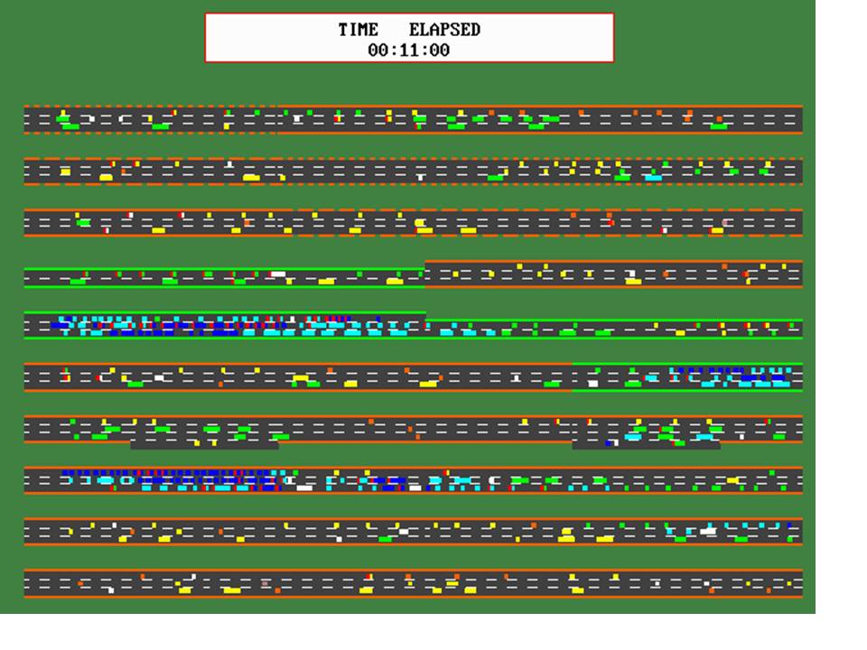
The model has a graphical display which allows the traffic flow to be viewed on-screen.  Figure 1 shows a typical view.  Vehicles enter at the bottom left and proceed from left to right along each of ten segments of the display, exiting at the top right.  The colour of the carriageway edges indicates the speed limit in force along a given section.  If the edge is dotted it indicates an uphill gradient, while a dashed edge indicates a downhill gradient.  The colour of the vehicles similarly indicates their speed.  The length of the vehicles reflects their physical length.  Ramps are indicated by a short extra lane adjacent to Lane 1 with no coloured edge.  The display indicates driving on the right, but this is not implicit in the model.  The inclusion of the graphical display was crucial for solving some of the more obtuse modelling and coding problems.  It also provides a good indication of the progress of a particular simulation.  Output is provided to a file for printing at pre-selected intervals.  The output data indicate flow rates, average speed, density, etc.

If this equation is assumed, it is still theoretically possible that de Sitter apparitions could be observed, but the distances involved would be much greater, to the extent that it is unlikely that they could ever be resolved. 

3.  The Driver Algorithm

The driver algorithm is central to the whole simulation.  The iterative loop begins by adding a vehicle at the beginning of the first section if required.  Each vehicle is checked for the completion of a lane change movement and then the crash status is verified.  If the vehicle has not crashed driver action follows, otherwise the vehicle will slow down and eventually stop.  After the driver action has been completed for all vehicles, their speeds are updated and the new position of each vehicle is calculated.  The speed of vehicles is recorded by means of energy accounting.  At this stage a new vehicle is added to any on-ramps if required, after which the vehicles are sorted and any new crashes recorded.  Finally, vehicles which have left the model, either by reaching the end of the model or via the off-ramps, are removed.  Any crashed vehicles are removed if the crash removal facility is invoked. 

The driver algorithm begins by calculating the 'safe' distance, Ss, for each driver.  This is given by

where S_s is given in metres, v is the instantaneous speed in metres per second and F is the safety factor for the driver group.  The actual distance behind the preceding vehicle, S_act, is the difference in their positions less the length of the leading vehicle.  An adjustment distance, S_adj is calculated using the braking deceleration, f, of the rear vehicle and the relative speeds, v₁ and v₂, of the two vehicles:

The key test is based on whether the actual distance is greater than the safe distance plus the adjustment distance.  If this is the case then the vehicle will attempt to move to a higher lane to overtake.  Failing that, it will slow down to avoid a rear end collision.  The order of decisions for each vehicle is as follows:

1. Calculate the 'safe' distance
2. If approaching an off-ramp and selected for exit, check to begin signalling to move in to a lower lane;
3. If signalling, attempt to change lanes;
4. Check ahead for lane closure and signal to move in if necessary, or bar moving to the closed lane;
5. Check for vehicles ahead in current lane (including double lane occupation for lane changes in progress);
6. Allow space, if possible, for vehicles signalling to move into current lane;
7. Allow space to move in if trying to exit;
8. Attempt to move to a higher lane to overtake if too close to vehicle in front;
9. If not following close to a preceding vehicle, attempt to move to a lower lane;
10. Look ahead for traffic moving freely in next lower lane and if so, attempt to move into it;
11. Calculate target speed;
12. Calculate new speed (but do not update speed until later).

The target speed is either the highest speed at which the driver would normally drive, or the maximum safe speed, if that is lower.  The maximum safe speed is the solution to the quadratic equation

Where S_adj and S_s are defined by Equations 1 and 2.

The speed adjustment attempts to achieve the target speed, either by either braking or accelerating.  Deceleration due to drag is calculated before any decision to brake is made.  If a reaction delay has been specified, a time delay must elapse before braking or acceleration can take place.  Braking is indicated by the operation of brake lights, which are indicated on the on-screen display.  The operation of brakes lights by the preceding vehicle causes a driver to reduce the estimate of the actual distance, S_act by 20%.

4.  Model Parameters

Many model parameters are under the control of the experimenter.  The model times used for most of the calculations reported here were a 1 hour run to allow flow to stabilise followed by a 2 hour run to minimise stochastic noise.  Eight vehicle types were used as shown in Table 1.  The maximum speed refers to the maximum attainable speed on a level road.  A drag factor is calculated assuming that the maximum power is deployed to obtain the maximum speed.  The drag factor is used to calculate the deceleration which occurs when no power is applied and the brakes are not applied.  The distribution of characteristics are the authors own estimate and are not based on traffic census data.  However, early sensitivity trials have shown that the calculations are not particularly sensitive to moderate variations in the value of these parameters.

Drivers were divided into five categories as shown Table 2.  Once again these are based entirely on the author's own estimates from observations.  The author is a member of the Institute of Advanced Motorists and thus claims to have some skill in assessing driving behaviour.  Once again, sensitivity trials have shown that the calculations are not particularly sensitive to moderate variations in the choice of parameter values.  No correlation is assumed between driver types and vehicle types.

The assignation of lanes and ramps is shown for each of the sets of calculations.  A 70  mph speed limit was chosen for all road sections where no speed restriction was required to restrict the flow.  This is the normal speed limit in the UK for this type of road.  The limit may vary somewhat from country to country, but, once again, the calculations are not sensitive to moderate variations in speed limit.  The timestep used was 0.5 s, except for the on-ramp calculations where 0.4 s was used and 5 lanes, where a 0.4 s timestep was required to achieve main flow saturation.  The off-ramp 5-lane calculations used a 0.25 s timestep.  Variations within these ranges are not critical to the calculations provided the timestep is sufficiently small to allow saturation to be reached.  No reaction delay was included because, with a 0.5 s timestep , a 0.5 s reaction time could lead to a 2 second delay in lifting off the accelerator and applying the brakes.  Clearly for the 'normal', 'impatient' and 'aggressive' drivers, this leads to an unrealistic profusion of collisions.  Crashed vehicle removal was enabled, although only 12 collisions were recorded in ~1000 km hours of calculations.  The maximum value for random adjustments was used to prevent "cloning", which could lead to platoons of vehicles all travelling at the same speed blocking all lanes of the highway to overtaking traffic.  The variations involved are quite small, with a maximum of ~10%.

5.  Vehicle Flow Rates

In the past, models of traffic flow have been created using either hydrodynamic models [1], the car following model [2] or cellular automata (see e.g. [3]).  Mishalani [4] has given some information, via the internet, of a model which appears to have similarities to the VEDENS model, but no details or references have been made available.  Previous workers have reported what they claim to be the fundamental flow diagram, which relates flow rates to vehicle density.  In terms of any infinite model or model with periodic boundary conditions, this arises because the density is pre-set and the model is then allowed to reach equilibrium, when it predicts the maximum safe speed which can be achieved for the pre-set density.  This represents an artificial constraint on the traffic flow.  In reality, vehicles enter a length of multilane highway either at the beginning or via on-ramps.  Neglecting on-ramps for the moment, the arrival rate will lead to a given flow rate along the highway.  If there are no constraints to the flow, such as obstructions, lane closures, ramps or speed limits, the traffic will move freely.  The density will increase until the maximum flow rate capacity of the road is achieved.  It is impossible to further increase the density without imposing some constraint on the flow.  The imposition of a constraint, such as a speed limit will further increase the density, and eventually lead to a reduction in the flow rate.  Thus the so-called fundamental diagram actually describes two independent physical phenomena. 

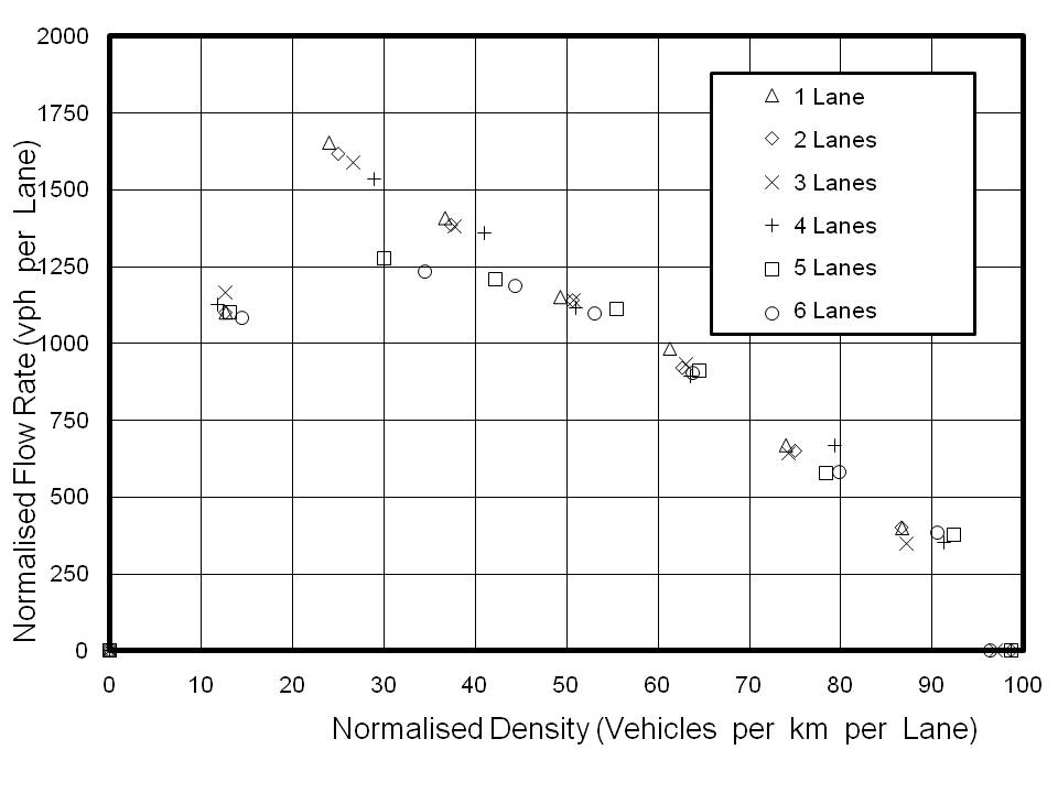
The calculations were made using a model of 2 km in length.  The final 500 m was assigned an appropriate speed limit for the flow restricted calculations (see below) in order to generate the required density.  Because the concept of the fundamental diagram is so well established, the effects of the two processes have been plotted as a single function.  The results are shown in Figure 2.  The flow to the left of the peak was generated by restricting the entry rate to the model.  Saturation is achieved when an increase in the attempted entry rate results in no increase in the actual flow rate within the model.  The flow to the right of the peak was generated by imposing a speed limit on saturated flow in the model.  The results are similar for all lane configurations, but the peak shifts to the right, broadens and is reduced in amplitude as the number of lanes increases.  This indicates that the capacity of a multilane highway is approximately proportional to the number of lanes, as could be predicted intuitively, but that for more than 4 lanes the relationship begins to break down.  The shift and flattening may be caused by the increased opportunity for lane changing, but no analysis has been carried out on this phenomenon at this stage.  There is also a shortening and steepening in the tail, as the speed approaches zero.  Once again this requires further consideration.  It is interesting to note that, in every case, the speed limit had to be reduced to as low as 20 mph in order to generate the first data point to the right of the peak.  At speeds higher than 20 mph the speed limit has almost no effect on the flow rate.  Thus it is deduced that practical speed limits alone will have no measurable effect on flow rate unless other factors, such as ramp flow, are taken into account. 

6.  On-Ramp Calculations

On-ramp perturbations have long been considered to be of significance in the creation of density nodes [5].  Because the ramp flow is generated as a proportion of the main flow, an off-ramp was also included to remove the main flow for the calculation with zero main flow.  Otherwise, the off-ramp played no part in the calculations.  The model was 2.2 km long and the ramp was 200 m in length, with vehicles being introduced at rest 50 m along the ramp.

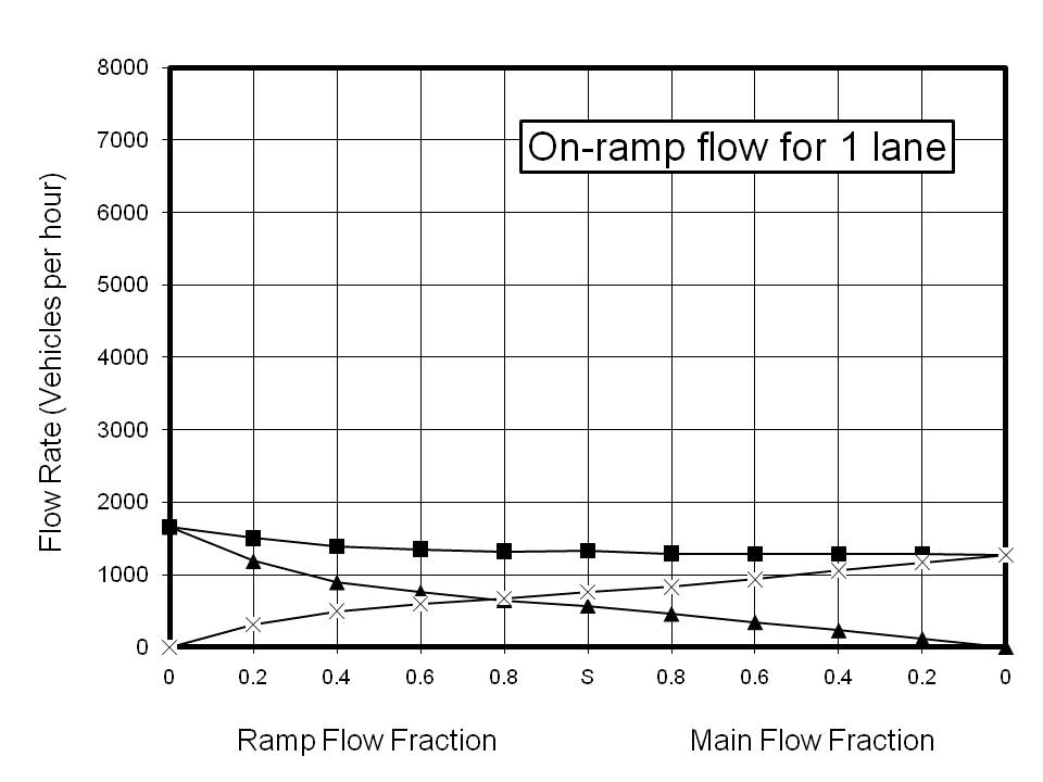
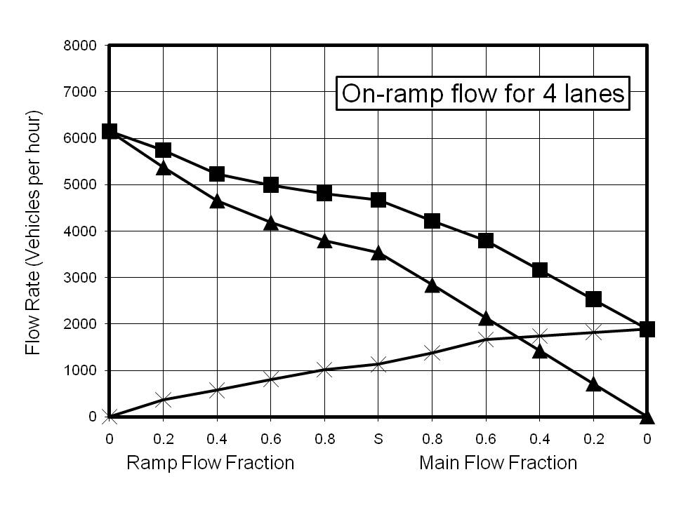
The results for on-ramp calculations are shown in Figure 3.  Calculations were performed for 1 to 5 lanes.  As with the fundamental diagram, these plots are composites of two different phenomena.  Point S on the x-axis represents saturated flow both for the input to the model and on the ramp.  The values of the flow rates were chosen to exceed the maximum achievable, and thus the flow rates are limited by the capacity of the road.  To the left of Point S, the main flow has been maintained as saturated and the ramp flow reduced to the indicated fraction of the saturated fraction.  Thus if the saturated fraction was 25% of the main flow the fraction indicated by 0.8 is 20% of the main flow.  To the right of Point S, the ramp flow has been maintained as saturated while the main flow was reduced to the indicated fraction of its saturated value.

The results for the 1-lane calculations are restricted by the low saturation value for 1-lane flow and are shown for reference only.  The striking feature of all the other reported results is that the saturation value for the ramp flow is very insensitive to the number of lanes.  Indeed, the total ramp flow possible with no main flow shows almost no increase corresponding with an increase in the number of lanes.  However, there is a very good correlation between the number of lanes and the main flow rate.  There are two clear conclusions which can be drawn from this.  The first is that increasing the number of lanes is an effective way of absorbing on-ramp flow.  For example the 3-lane calculation indicates that the maximum main flow rate of ~4800 vehicles per hour (vph) is reduced to ~2500 vph when the on-ramp flow reaches ~1000 vph.  However, the prediction for a 5-lane highway indicates that a main flow rate of ~5000 vph is possible for the same ramp flow. 

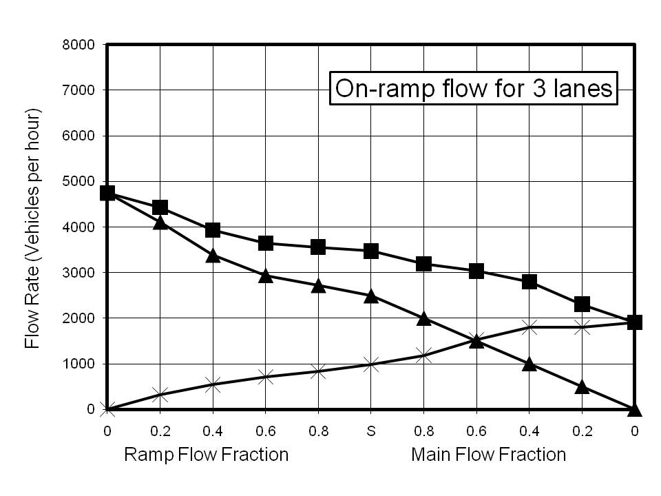
The second implication is that multiple ramps, such as those with two separated lanes, are capable of increasing the ramp flow, providing there is sufficient capacity for the main flow.  Reference to the results for the 3-lane calculation illustrates this point.  If the main flow is less than ~1500 vph then two on-ramps, each with a flow of ~1000 vph would not overload the highway.  However, the saturated total capacity at an on-ramp is predicted to be ~3500 vph, so if the main flow were initially higher than ~1500 vph, the main flow approaching the on-ramp would become restricted, resulting in severe congestion and a 'tail-back' of slow moving or stationary vehicles.

7.  Off-Ramp Calculations

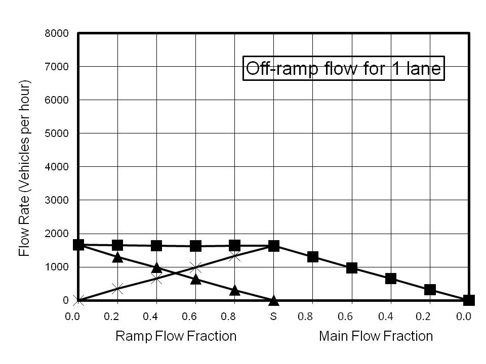
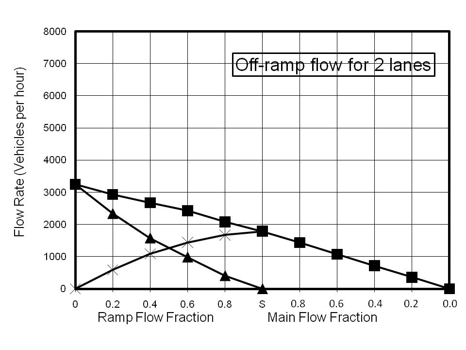
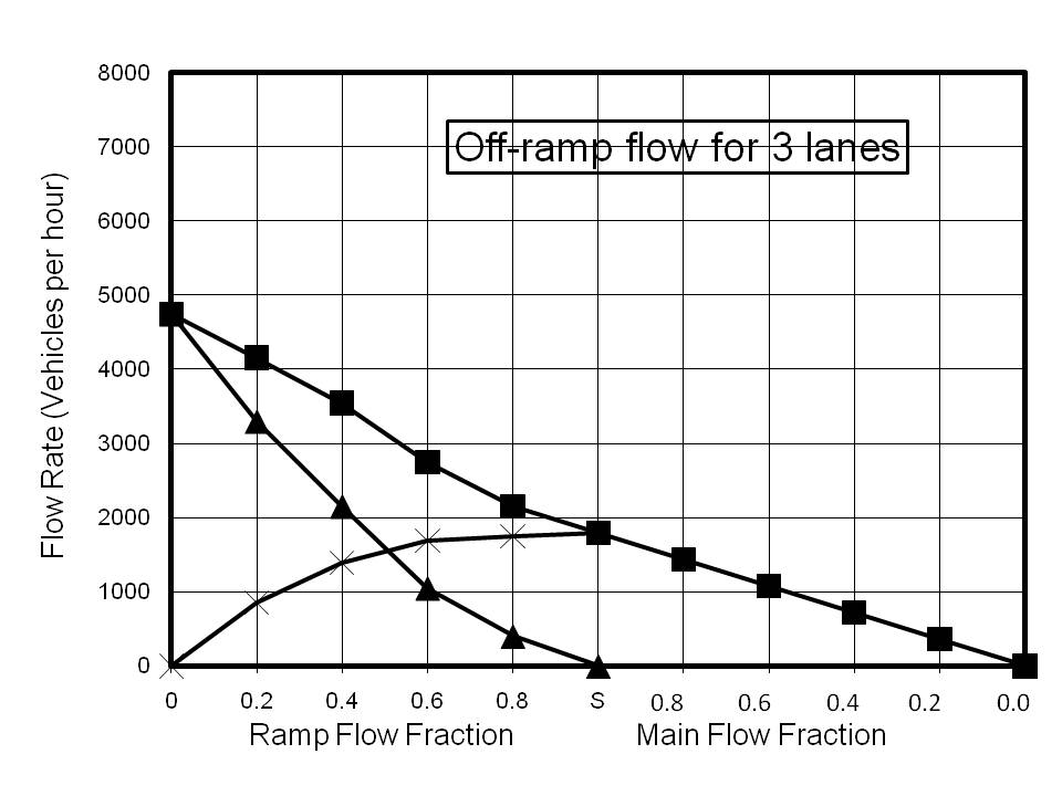
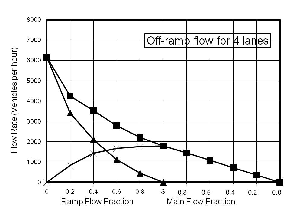
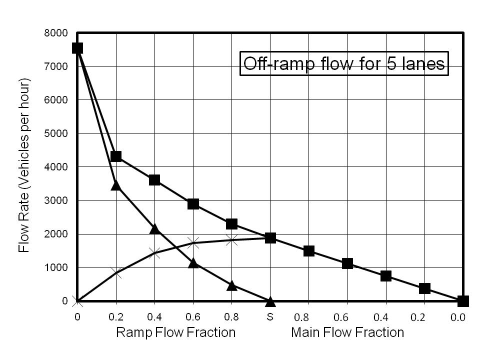
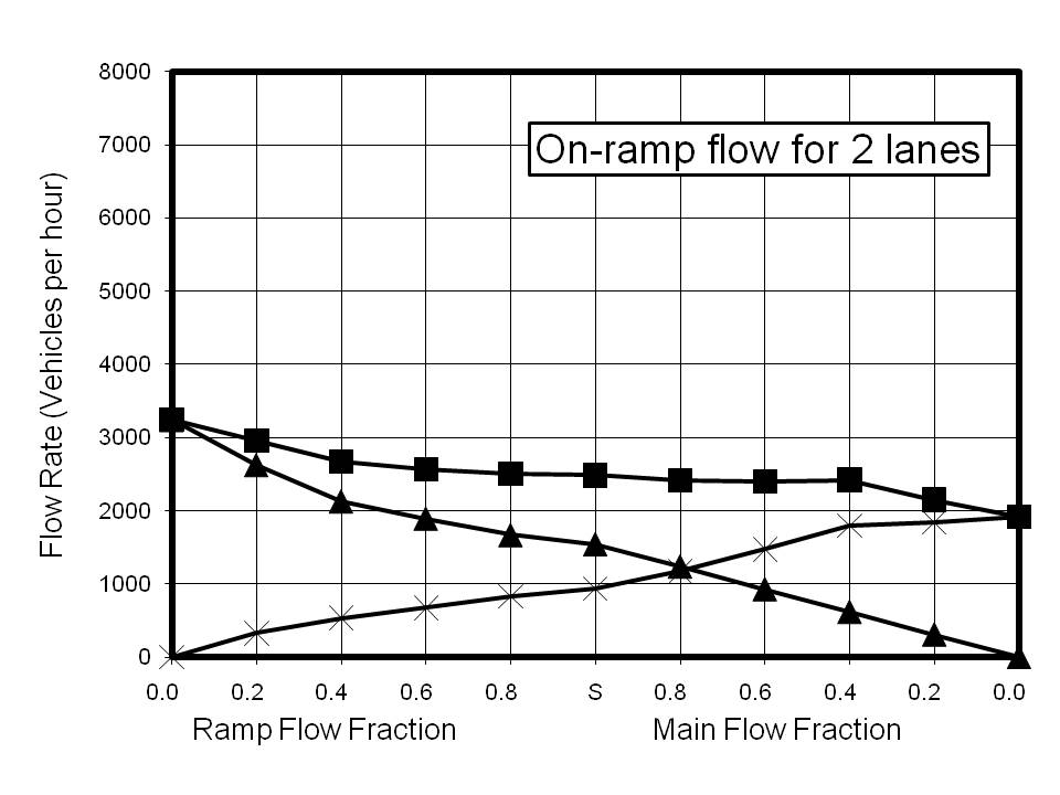
There is little reference in the literature to off-ramp perturbations as a significant factor in the creation of density nodes.  As with the on-ramp calculations, the model was 2.2 km long and the ramp was 200 m in length.  Vehicles are deleted 20 m before the end of the ramp.  The results for off-ramp calculations are shown in Figure  4.  Once again these plots are composites of two different phenomena.  Point S on the x-axis represents saturated flow for the input to the model with the entire flow being diverted to the ramp.  The values of the main flow rates were chosen to exceed the maximum achievable, and thus the flow rates are limited by the capacity of the road To the left of Point S, the main flow has been maintained as saturated and the ramp flow set to the indicated fraction of the main flow.  The decision whether or not to leave the highway via the off-ramp is made at ~1.4 km before the ramp, by comparing the desired fraction with a random number generated from a uniform distribution between 0 and 1.

As with the on-ramp calculations, the saturation value for the ramp flow is very insensitive to the number of lanes.  Even more striking is the fact that with ramp flows of greater than 20%, the model predicts that there is no advantage in building a highway with more than 3 lanes.  It can be seen that for a 3-lane highway ~4200 vph can be accommodated with a 20% off-ramp exit rate, which is almost identical to the saturated flow rate for 5 lanes with the same exit rate.  At first sight this is indeed a surprising result.  However, the phenomenon of slow moving traffic nodes is frequently encountered for some distance prior to off-ramps when flow rates are high.  The explanation is almost certainly that traffic changing to a lower lane in preparation for an exit slows the existing traffic in that lane.  Consequently, vehicles not wishing to exit may change to a higher lane, causing congestion in the higher lanes.  Clearly, the more lane changes are involved to make an exit, the more significant will be the effect.  Thus on a 5-lane highway the average number of lane changes to exit, assuming an even distribution of exiting vehicles across the 5 lanes is two, whereas for a 3-lane highway the average is only one.

8.  Highway Blockage

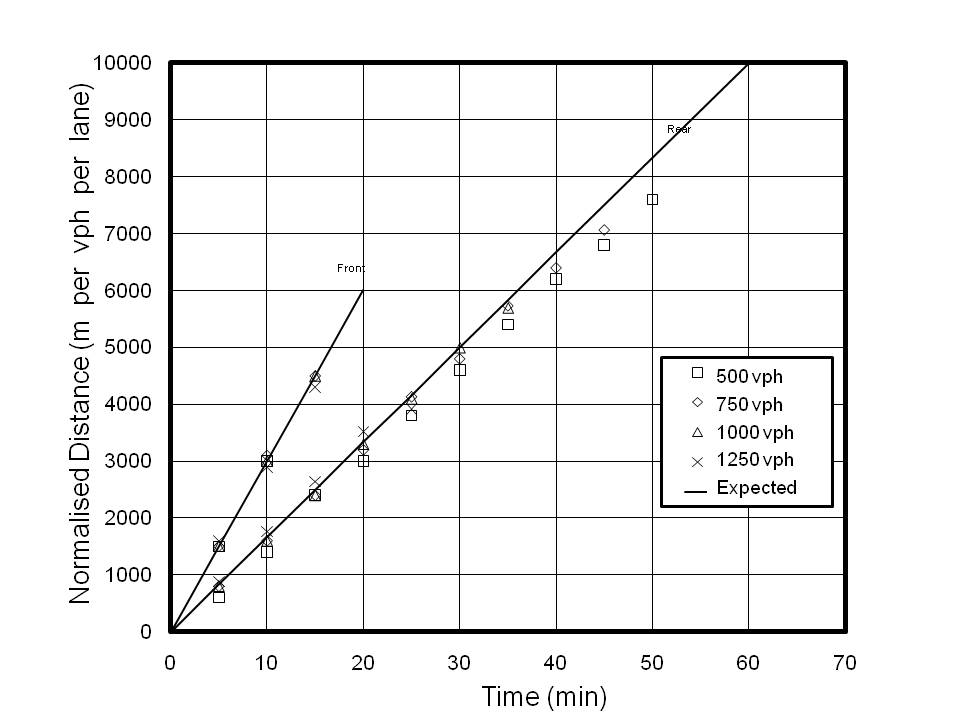
The following arguement assumes that there is a discontinuous transition between the flow rate within a node and the flow rate outside it.  If the highway becomes totally blocked, for example because of an accident, or to allow the emergency services to carry out a manoeuvre, traffic will come to a complete standstill and a tailback will be created.  If the traffic flow rate is R vph, the mean vehicle length L m, including the mean inter-vehicular gap and the number of lanes is n, the tailback will grow at the rate, T'_r, given by

So, after t₁ minutes, the tail back will stretch to RLt₁/60n m.  If the blockage is removed at t₁ minutes, the leading vehicles will begin to move away from the stationary node at the maximum flow capacity of the highway, R_max and so the front of the node will move back along the highway at a rate T'_f

So, after t₂ minutes, the front of the node will be

from the original point of the blockage and the length of the tailback L_tb will be

When L_tb = 0 we have

and the point at which the stationary node disappears will be

from the position of the original blockage.  Clearly, if R is small compared with R_max, the tailback will be relatively small and the node will disappear in a short time.  However, as R approaches R_max, the length of the tail back and the time for it to clear will increase significantly.  As it disappears, the stationary node will be transformed into a moving node.  The flow rate within the node will be R_max, whereas the flow rate of traffic approaching the rear of the node will be R.  The speed of the trailing edge of this moving density node can be calculated with reference to the mean speed of the vehicles in the node v₂ and the mean speed of the vehicles approaching the trailing edge of the node v₁.  If v₂ = xv₁, such that v₂ < v₁ and R = yR_max, it can be shown that the speed of the trailing edge of the density node, v_trail, is

which is less than v₂.  A similar arguement can be made for the leading edge of the moving density node, except that initially, the flow rate of the traffic in front of the node is very low (increasing from zero) and the mean velocity will be that associated with low traffic densities.  Thus it can be seen that the density node would be expected to travel in a positive direction, but at a slower speed than the mean speed of the vehicles in the node.

In reality, the transition is not discontinuous because vehicles approaching the rear of a node will slow down as they approach, while vehicles at the front will accelerate as the road ahead becomes clear.  However if the stationary node is regarded as all vehicles travelling at less than 10 mph, Equations 4 and 5 hold reasonably well. 

Figure 5 shows the results for 3-lane calculations, with the results for all flow rates normalised for comparison.  Calculations for other lane configurations rendered similar results, although the front edge of the node moved slightly faster for 1- and 2-lane calculations at the lower flow rates. 

9. Conclusions

The VEDENS computer code has been tested using sample distributions judged by the author to be reasonably representative of typical traffic conditions on major routes within the UK mainland.  The driver algorithm could form the basis of a rudimentary automatic vehicle control system.  The code has reproduced many observed phenomena, such as packing in the highest lane when flow rates approach the maximum capacity of the highway and queuing in lanes approaching a flow restriction, such as a ramp or lane closure.  Four types of phenomena have been investigated.

Maximum Flow Rates: The calculations have show that the maximum achievable flow rate (capacity) of a multilane unidirectional highway is approximately proportional to the number of lanes.  However the efficiency (i.e.  the capacity per lane) decreases slightly as the number of lanes increases.  For up to 3 lanes the decrease in efficiency is small, but for 5-and 6-lane configurations there is a marked decrease.  Reducing the speed limit has little effect on the flow rate for speeds of greater than 20 mph.  At lower speeds, the flow rate will be reduced.

On-ramps: Increasing the number of lanes increases the capacity of the highway at the approach to an on-ramp.  However, it has little effect on the ramp capacity.  It is expected that the ramp capacity could be increased by using ramps with separated lanes (effectively ramps in tandem), but no calculations have been carried out for this configuration to date.

Off-ramps: Increasing the number of lanes increases the capacity of the highway at the approach to an off-ramp under certain conditions.  However, in situations where 20% or more of the traffic wishes to leave via a given off-ramp, increasing the number of lanes to more than 3 has little effect.  This is almost certainly caused by the manoeuvring required for vehicles to move into Lane 1 in readiness for exiting via the ramp.

Blockages: When the highway is completely blocked for a short period of time, such as after a minor incident, a density node of stationary or very slow moving traffic will form.  The behaviour of the leading and trailing edges of the node can be predicted quite well by simple equations.  However, once the speed of the traffic within the node increases, the node appears to disperse and the behaviour is more difficult to characterise.

References

[1] I Prigogine and R Herman in: Kinetic Theory of Vehicular Traffic Elsevier New York (1971)
[2] L Eisenburg and E Caplan An investigation of the Car-Following Model using Continuous System Model Program (CSMP) Techniques University of Pennsylvania UMTA-URT-8(70)-71-04 (1971)
[3] P Wagner, K Nagel and D E Wolf Physica A 234 (1996) p687
[4] Information taken from: http://web.mit.edu:1962/tiserve.mit.edu/9000/41350.html (1995)
[5] P K Munjal and L A Pipes Transport Science 5 (1991)